@misc{llm-scaling-laws-paper-excerpt-scaling-laws-for-neural-language-models,
  author = {Jingxi Qiu},
  title = {LLM Scaling Laws Paper Excerpt - Scaling Laws for Neural Language Models},
  howpublished = {Jingxi Qiu},
  year = {2024},
  url = {https://mouwumou.github.io/blog/llm-scaling-laws-paper-excerpt-scaling-laws-for-neural-language-models/}
}

Qiu, J. (2024). LLM Scaling Laws Paper Excerpt - Scaling Laws for Neural Language Models. In Jingxi Qiu.

Qiu, Jingxi. “LLM Scaling Laws Paper Excerpt - Scaling Laws for Neural Language Models.” Jingxi Qiu, 2024.

Qiu, Jingxi. 2024. “LLM Scaling Laws Paper Excerpt - Scaling Laws for Neural Language Models.” In Jingxi Qiu. Preprint.

✋ Many people believe that the performance of large models is related to the model's structure, size, training compute, and dataset size. However, how exactly do these factors influence the final performance of a large model? Understanding this can help in better deciding where to invest resources to train the required models.

Background and Content#

In 2020, OpenAI released the paper "Scaling Laws for Neural Language Models," exploring Scaling Laws. This paper discusses the relationship between the training loss of large models based on Transformers and the model parameter size (N), dataset size (D), and computational volume (C).

In April 2022, Google DeepMind revisited Scaling Laws in their article "Training Compute-Optimal Large Language Models." They pointed out that current large models are significantly under-trained. By using four times the data (compared to the 280B parameter Gopher) to train the 70B parameter Chinchilla, they achieved better results (SOTA average accuracy of 67.5% on the MMLU benchmark, a 7% increase).

However, in February 2023, a blog titled "Chinchilla’s Death" by Thaddée Tyl argued that with sufficient training time, small models can outperform large models.

Paper#

Scaling Laws for Neural Language Models#

Key Findings#

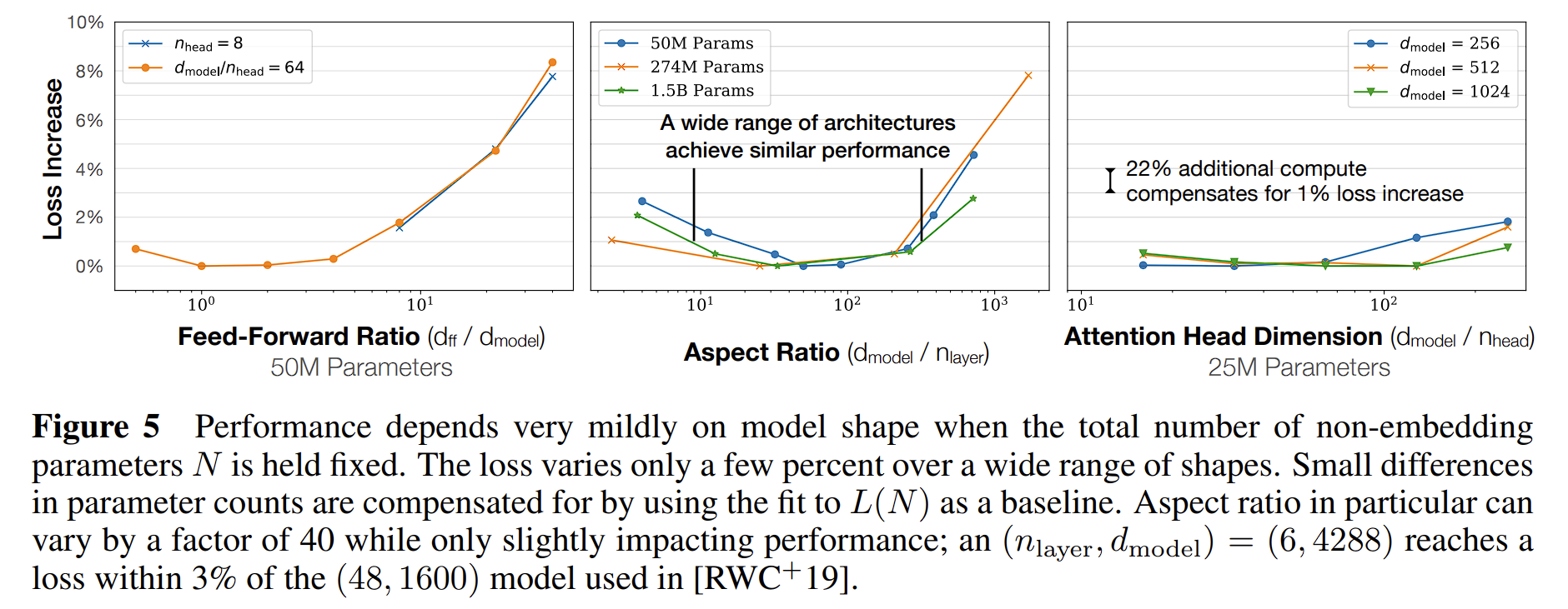
1. Model performance improves with the increase in model size (N), dataset size (D), and compute (C), and is weakly correlated with the model's shape (depth and width) and the number of self-attention heads.
2. When other factors are not limited, there is a power-law relationship between model size (N), dataset size (D), compute (C), and performance.
3. Expanding both model size (N) and dataset size (D) simultaneously can improve model performance. However, the study suggests that when the model size increases eightfold, the dataset size only needs to increase fivefold, and this will not incur a performance penalty.
4. Because the training curve follows a power-law relationship, the loss is independent of model size, allowing us to roughly predict the loss for subsequent training.
5. There is a penalty (greater error) when transferring to a dataset different from the training set, but this penalty is constant, meaning other improvements are consistent.
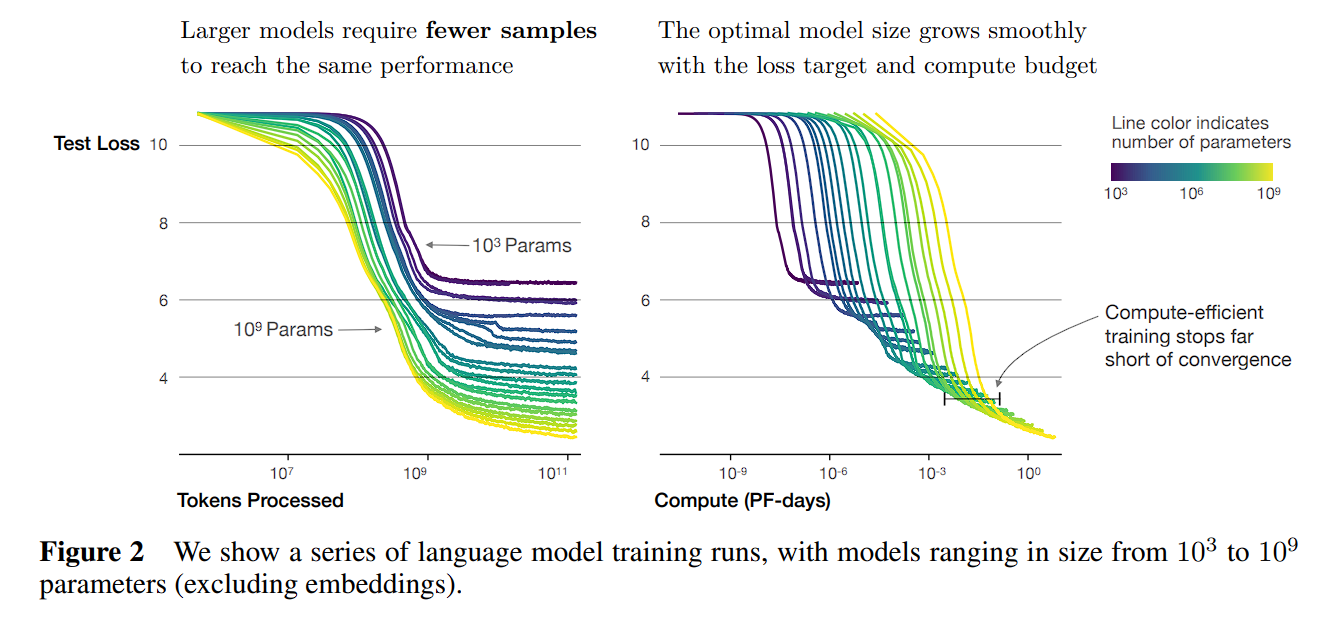
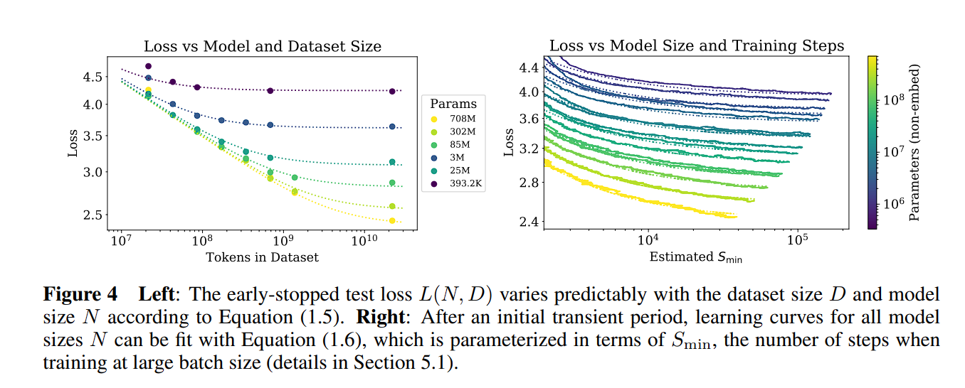
6. Large models have higher sample efficiency compared to smaller models, requiring less training (Figure 2) and less data (Figure 4) to achieve the same level of performance.

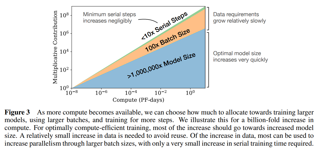
1. Convergence is inefficient. When the compute (C) is fixed, it is possible to stop training before the model fully converges to achieve optimal performance (Figure 3). The paper provides a reference relationship as follows: $D\sim C^{0.27}$

1. The ideal batch size for training should be proportional to the power of the training data size and can be further determined using the gradient noise scale.

Scaling Law Summary#

Parameters：

non-embedding parameters $N$

the dataset size $D$

optimally allocated compute budget $C_{min}$

When the other two factors are not limited, the test loss can be predicted using the following formula:

1. N is limited

$$\begin{equation} L(N)=(N_c/N)^{\alpha_N} \end{equation}$$ $$\alpha_N \sim 0.076,N_c \sim 8.8 \times 10^{13} \text{(non-embedding parameters)}$$

1. D is limited（with early stopping)

$$\begin{equation} L(D)=(D_c/D)^{\alpha_D} \end{equation}$$ $$\alpha_D \sim 0.095, D_c \sim 5.4 \times 10^{13}\text{(tokens)}$$

1. C is limited

$$\begin{equation}L(C_{min})=(C^{min}_c/C_{min})^{\alpha_{min}} \end{equation}$$ $$\alpha_C^{min} \sim 0.050, C^{min}_c \sim 3.1 \times 10^8 \text{(PF-days)}$$

Formula Meaning:

In the above formulas, $\alpha_N, \alpha_D, \alpha_C^{min}$ indicate the power law exponents that describe the performance improvement when increasing $N,D,C_{min}$.

For example, if we double the number of model parameters, the model loss will decrease by a factor of $2_{-\alpha_N}\approx 0.95$, meaning the loss will be 0.95 times the previous value. The exact numbers for $N_C,D_C,C_C^{min}$ are based on vocabulary size and tokenization, thus only representing an order of magnitude relationship rather than precise values.

Additionally, the paper discusses the relationship between batch size and loss.

$$\begin{equation}B_{crit}(L)=\frac{B_*}{L^{1/a_B}} \end{equation}$$ $$B_* \sim 2\cdot10^8 \text{tokens}, \alpha_B\sim0.21$$

Based on the previous formulas (1) and (2), when we increase the model size, we should correspondingly increase the dataset size. It can be calculated as:$D\propto N^{\frac{\alpha_{N}}{\alpha_D}} \sim N^{0.74}$。

They also derived a combined formula from (1) and (2) to manage the dependencies of N and D and to control overfitting:

$$\begin{equation}L(N,D)=\left[\left(\frac{N_c}{N}^{\frac{\alpha_N}{\alpha_D}}+\frac{D_c}{D} \right) \right]^{\alpha_D}\end{equation}$$

• The authors speculate that this function can also generate the maximum log-likelihood for other generative tasks.

The training curve can also be derived from the number of training steps, allowing us to determine the optimal number of training steps.

$$\begin{equation}L(N,S)=\left(\frac{N_c}{N}\right)^{\alpha{N}}+\left(\frac{S_c}{S_{min}(S)}\right)^{\alpha_S}\end{equation}$$

$S_c \approx 2.1 \times 10^3,\alpha_S \approx 0.76$ $S_{min}(S)$ is the minimum possible number of optimization steps (parameter updates) estimated using Equation

In the case of fixed compute C, the following relationship formula is derived:

$$\begin{equation}N \propto C^{\alpha^{min}_C /\alpha_N}, B \propto C^{\alpha^{min}_C /\alpha_B}, S \propto C^{\alpha^{min}_C /\alpha_S}, D = B \cdot S\end{equation}$$

Here we have:

$$\begin{equation}\alpha^{min}_C=1/(1/\alpha_S+1/\alpha_B+1/\alpha_N)\end{equation}$$

So we can get $N \propto C^{0.73}_{min}, B \propto C^{0.24}_{min},\text{ and }S \propto C^{0.03}_{min}$，here drop out the ideas：

1. When the compute budget C is increased, it should primarily be used to create larger models rather than extending training time or increasing dataset size.

2. Additionally, as models become larger, they become more sample efficient.

Research Methodology#

The study was conducted using the WebText2 dataset and its extension (2.29 × 10^10 tokens). The tokenization method employed was byte-pair encoding, with a vocabulary size of $n_{vocab}=50257$. The performance metric (Loss) was the cross-entropy loss over a context of 1024 tokens. The primary model used was a decoder-only Transformer, and LSTM along with other types of Transformers were also trained for comparison.

Unless otherwise specified, the model training utilized the Adam optimizer for $2.5 \times 10^5$ steps with a batch size of 512 and a context of 512 tokens. Due to memory constraints, the largest models were trained using the Adafactor optimizer.

The learning rate schedule, unless otherwise noted, included a warm-up period of 3000 steps followed by cosine decay to zero.

Model Parameter Calculation Method

To calculate the model parameters and compute requirements, the model hyperparameters are defined as follows:

$n_{layer}$	层数 number of layers
$d_{model}$	残差流的维度 dimension of the residual stream
$d_{ff}$	前馈层（全连接）的维度 dimension of the intermediate feed-forward layer
$d_{attn}$	注意力输出的维度 dimension of the attention output
$n_{heads}$	每层注意力头数量 number of attention heads per layer
$n_{ctx}$	上下文词元数量，除另说明外为1024 input context

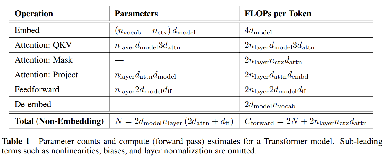
$N$ to represent the size of the model parameters, excluding the embedding layers, the calculation for model parameters is as follows:

$$\begin{aligned} N&\approx 2d_{model}n_{layer}(2d_{attn}+d_{ff}) \\ &= 12n_{layer}d^2_{model}\end{aligned}$$ $$d_attn=d_{ff}/4=d_{model}$$

Here, the parameters for the embedding layers $n_{vocab}d_{model}$ and $n_{ctx}d_{model}$ are omitted.

The compute required for a forward pass, denoted as $C$, is approximately:

$$C_{forward} \approx 2N+2n_{layer}n_{ctx}d_{model}$$

Experimental Results#

Experimental Variables:

• Model Size: Ranging from 768 non-embedding parameters to 1.5 billion parameters.
• Dataset Size: From 22 million to 23 billion tokens.
• Model Shape: Including variations in depth, width, attention heads, and feed-forward dimensions.
• Context Length: Typically 1024 tokens, but shorter contexts were also tested.
• Batch Size: Typically $2^{19}$, but varied to measure the critical batch size.

Conclusion:

1. When the non-embedding model size $N$ is fixed, the model shape has a minimal impact on performance, with large adjustments affecting performance by only a few percentage points.
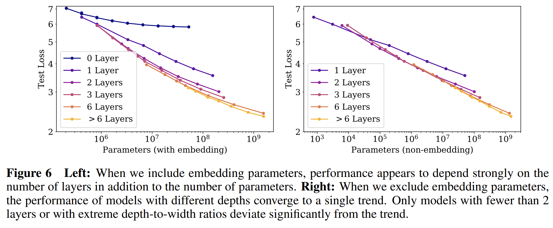
2. If the embedding parameters are included, model performance shows a significant correlation with the number of layers (left graph). However, if the embedding parameters are excluded, the performance of models with different numbers of layers follows the same trend, except for models with fewer than two layers (right graph).
3. The same applies to LSTM models, although LSTM performance is slightly inferior to Transformers.
4. The power law theorem formula holds:

$$\begin{align}L(N)&\approx(N_c/N)^{\alpha_N} \\ L(D)&\approx (D_c/D)^{\alpha_D} \\ L(C_{min})&\approx(C^{min}_c/C_{min})^{\alpha_{min}} \end{align}$$

参考#

[1] https://arxiv.org/pdf/2001.08361.pdf

[2] https://arxiv.org/pdf/2203.15556.pdf

[3] https://espadrine.github.io/blog/posts/chinchilla-s-death.html

[4] https://arxiv.org/pdf/2109.10686.pdf

[5] https://self-supervised.cs.jhu.edu/sp2023/files/17.retrieval-augmentation.pdf